Transformer原理以及文本分类实战 |
您所在的位置:网站首页 › transform encoder › Transformer原理以及文本分类实战 |
Transformer原理以及文本分类实战
|
目录
1. Model2. Encoder2.1 Position encoding2.2 Multi-Head AttentionAdd&NormFeed forward
3. Decoder4. 源码解读(pytorch)5. 文本分类实战参考
1. Model
在此之前,假定你已经了解了:RNN(LSTM),Sequence2Sequence模型以及注意力机制。Transformer通过大量使用Attention代替了Seq2seq中的RNN结构,使得整个模型可以并行计算(RNN只能等待t-1时间步计算完成才能计算下一个时间步t)。 正如所有的Seq2seq一样,整个模型也分为Encoder以及Decoder两部分(分别对应图中的左边和右边)。 Encoder部分使用了Nx=6个相同的Block,每个Block可以拆解为如下四个部分: 因为Transformer没有RNN中的顺序结构,因此需要加入单词的位置信息来显示地表明单词上下文关系。论文中使用了下面的式子来进行位置嵌入: 下面生成的heat map很好地展示了函数的周期性。每一行都对应了一个position encoding,并且随着行列的增加,其变化的周期都在逐渐增加。因此每一个POS和i产生的位置信息都是不同的。 这部分的详解可以参见一个知乎的帖子:https://zhuanlan.zhihu.com/p/47282410。attention函数可以看作将一个query和一系列key-value对映射为一个输出(output)的过程。 Add表示残差连接,为了防止模型过深带来的梯度消失或梯度爆炸问题。 两次线性变换之后并经过relu激活函数,之后重复Add&Norm之中的操作。 同Encoder一样,Decoder也有6层,只不过在最开始多了一个Mask的多头注意力,这个确保了pos位置的预测结果只能取决于pos之前的预测结果。 4. 源码解读(pytorch)由于只关注文本分类任务,所以代码中只包含Encoder的实现。代码借鉴了github上的一位大佬,https://github.com/649453932/Chinese-Text-Classification-Pytorch/blob/master/models/Transformer.py 我们先规定输入的三维张量为x。 然后,我们去实现上边的提到的部件。第一个是Positional_Encoding。 class Positional_Encoding(nn.Module): ''' params: embed-->word embedding dim pad_size-->max_sequence_lenght Input: x Output: x + position_encoder ''' def __init__(self, embed, pad_size, dropout): super(Positional_Encoding, self).__init__() self.pe = torch.tensor([[pos / (10000.0 ** (i // 2 * 2.0 / embed)) for i in range(embed)] for pos in range(pad_size)]) self.pe[:, 0::2] = np.sin(self.pe[:, 0::2]) # 偶数sin self.pe[:, 1::2] = np.cos(self.pe[:, 1::2]) # 奇数cos self.dropout = nn.Dropout(dropout) def forward(self, x): # 单词embedding与位置编码相加,这两个张量的shape一致 out = x + nn.Parameter(self.pe, requires_grad=False).cuda() out = self.dropout(out) return outMulti-Head Attention class Multi_Head_Attention(nn.Module): ''' params: dim_model-->hidden dim num_head ''' def __init__(self, dim_model, num_head, dropout=0.0): super(Multi_Head_Attention, self).__init__() self.num_head = num_head assert dim_model % num_head == 0 # head数必须能够整除隐层大小 self.dim_head = dim_model // self.num_head # 按照head数量进行张量均分 self.fc_Q = nn.Linear(dim_model, num_head * self.dim_head) # Q,通过Linear实现张量之间的乘法,等同手动定义参数W与之相乘 self.fc_K = nn.Linear(dim_model, num_head * self.dim_head) self.fc_V = nn.Linear(dim_model, num_head * self.dim_head) self.attention = Scaled_Dot_Product_Attention() self.fc = nn.Linear(num_head * self.dim_head, dim_model) self.dropout = nn.Dropout(dropout) self.layer_norm = nn.LayerNorm(dim_model) # 自带的LayerNorm方法 def forward(self, x): batch_size = x.size(0) Q = self.fc_Q(x) K = self.fc_K(x) V = self.fc_V(x) Q = Q.view(batch_size * self.num_head, -1, self.dim_head) # reshape to batch*head*sequence_length*(embedding_dim//head) K = K.view(batch_size * self.num_head, -1, self.dim_head) V = V.view(batch_size * self.num_head, -1, self.dim_head) # if mask: # TODO # mask = mask.repeat(self.num_head, 1, 1) # TODO change this scale = K.size(-1) ** -0.5 # 根号dk分之一,对应Scaled操作 context = self.attention(Q, K, V, scale) # Scaled_Dot_Product_Attention计算 context = context.view(batch_size, -1, self.dim_head * self.num_head) # reshape 回原来的形状 out = self.fc(context) # 全连接 out = self.dropout(out) out = out + x # 残差连接,ADD out = self.layer_norm(out) # 对应Norm return outscaled Dot-Production class Scaled_Dot_Product_Attention(nn.Module): '''Scaled Dot-Product''' def __init__(self): super(Scaled_Dot_Product_Attention, self).__init__() def forward(self, Q, K, V, scale=None): attention = torch.matmul(Q, K.permute(0, 2, 1)) # Q*K^T if scale: attention = attention * scale # if mask: # TODO change this # attention = attention.masked_fill_(mask == 0, -1e9) attention = F.softmax(attention, dim=-1) context = torch.matmul(attention, V) return context最后一个部件是Feed Forward class Position_wise_Feed_Forward(nn.Module): def __init__(self, dim_model, hidden, dropout=0.0): super(Position_wise_Feed_Forward, self).__init__() self.fc1 = nn.Linear(dim_model, hidden) self.fc2 = nn.Linear(hidden, dim_model) self.dropout = nn.Dropout(dropout) self.layer_norm = nn.LayerNorm(dim_model) def forward(self, x): out = self.fc1(x) out = F.relu(out) out = self.fc2(out) # 两层全连接 out = self.dropout(out) out = out + x # 残差连接 out = self.layer_norm(out) return out然后看整体的Encoder实现: class Encoder(nn.Module): def __init__(self, dim_model, num_head, hidden, dropout): super(Encoder, self).__init__() self.attention = Multi_Head_Attention(dim_model, num_head, dropout) self.feed_forward = Position_wise_Feed_Forward(dim_model, hidden, dropout) def forward(self, x): out = self.attention(x) out = self.feed_forward(out) return out 5. 文本分类实战本文分类使用公开数据集mr,按照默认的方式拆分训练集与测试集。使用Stanford的Glove50将数据处理成上文提到的张量格式,对于不同的Sequence需要补全成相同的长度。 对于其它参数,配置如下: class ConfigTrans(object): """配置参数""" def __init__(self): self.model_name = 'Transformer' self.dropout = 0.5 self.num_classes = cfg.classes # 类别数 self.num_epochs = 100 # epoch数 self.batch_size = 128 # mini-batch大小 self.pad_size = cfg.nV # 每句话处理成的长度(短填长切),这个根据自己的数据集而定 self.learning_rate = 0.001 # 学习率 self.embed = 50 # 字向量维度 self.dim_model = 50 # 需要与embed一样 self.hidden = 1024 self.last_hidden = 512 self.num_head = 5 # 多头注意力,注意需要整除 self.num_encoder = 2 # 使用两个Encoder,尝试6个encoder发现存在过拟合,毕竟数据集量比较少(10000左右),可能性能还是比不过LSTM config = ConfigTrans() class Transformer(nn.Module): def __init__(self): super(Transformer, self).__init__() self.postion_embedding = Positional_Encoding(config.embed, config.pad_size, config.dropout) self.encoder = Encoder(config.dim_model, config.num_head, config.hidden, config.dropout) self.encoders = nn.ModuleList([ copy.deepcopy(self.encoder) for _ in range(config.num_encoder)]) # 多次Encoder self.fc1 = nn.Linear(config.pad_size * config.dim_model, config.num_classes) def forward(self, x): out = self.postion_embedding(x) for encoder in self.encoders: out = encoder(out) out = out.view(out.size(0), -1) # 将三维张量reshape成二维,然后直接通过全连接层将高维数据映射为classes # out = torch.mean(out, 1) # 也可用池化来做,但是效果并不是很好 out = self.fc1(out) return out结果分析: 在epoch=40设置learning rate decay,decay rate 0.97,并将early stop设置为20,损失函数使用pytorch自带的交叉熵。在epoch=51时early stop,mr准确率约为71%。对比BiLSTM+Attention的73.86%,准确率反而逊色。可能是因为transformer更适用于较大的数据集,mr的数据量还是比较小。 Epoch:51---------loss:34.51407927274704-----------time:8.6797354221344 epoch:51 test_acc:0.7062464828362408 best_acc:0.7121553179516038 early stop!!! Best acc:0.7121553179516038 参考https://www.bilibili.com/video/BV1sE411Y7cP?from=search&seid=2004285655536337633 https://www.jianshu.com/p/0c196df57323 https://blog.csdn.net/qq_29695701/article/details/88096455 |
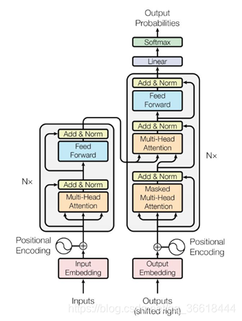 Encoder在给定一个sequence(x1…xn)的输入之后,将其映射到隐藏层H(h1…hn);Decoder以H为输入,一次一个字符地生成解码之后的结果(y1…ym),这里n不一定等于m。为了告知Decoder开始与结束,最初的输入是一个表示开始的特殊字符(这里假定是< START>),直到输出< END>为止。对于文本分类等下游任务,只需要用到Encoder部分即可。Bert也只用到了Encoder,因此我们把重点放在Encoder上。
 最开始的Inputs是我们经常能见到的三维张量:batch×sequence_length×embedding_dim。输出X_hidden和输入差不多。
 其中PE是一个二维矩阵,形状就是sequence_length×embedding_dim,pos是单词在句子中的位置,d_model表示词嵌入的维度,i表示词向量的位置。奇数位置使用cos,偶数位置使用sin。这样就根据不同的pos以及i便可以得到不同的位置嵌入信息,然后,PE同对应单词的embedding相加,输入给第二层。我们通过可视化的方式来验证这两个函数为什么能产生不同的位置信息:
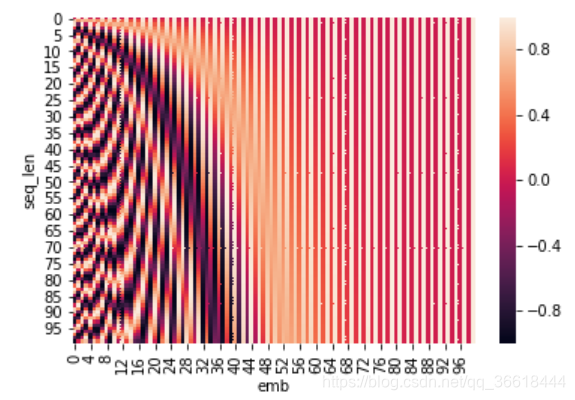
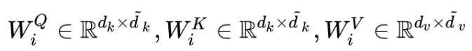
 self-attention的具体结构如左图所示,首先,通过对初始输入X做三种不同的线性变换我们得到大家耳熟能详的KQV:Q = WQ X ; K = WK X ; V= WV X。 之后,通过scaled Dot-Production得到输出,其中dk是词向量的维度,除以dk1/2 的这个操作也就是所谓的scaled。这个操作是为了使softmax之后的结果变得更稳定。Q与KT的结果是一个n×n的矩阵,表示这句话中每个单词对于其它任意单词的注意力。然后再乘V(初始输入X变换之后的特征值),就得到了注意力加权之后的特征,这个特征相比于X,维度并没有任何变化。
 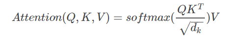 Mask的作用是在计算softmax的时候对padding的部分进行屏蔽,避免了这部分无用信息对后面的影响。 接下来就是论文中的核心Multi-Head Attention部分了。Multi-Head Attention就是把上述的过程的过程做H次,然后把输出拼接起来。论文中采用了对KQV进行分割的方式实现多头注意力,也就是把shape为batch×sequence_length×embedding_dim的三个张量reshape成【batch×sequence_length×head×embedding_dim//head】,因此在代码实现的过程中也必须要注意head数必须能够被词嵌入的维度整除。 公式描述如下:
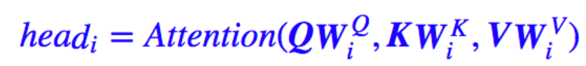

 norm则表示Layer Normalization。
【本文地址】